Follow my journey in learning Advanced Statistics with all the content, tricks, and lessons learned!
Module 12: Timely Time Series
Get link
Facebook
X
Pinterest
Email
Other Apps
Hi everyone!
This week we are looking into time series where we dive into the past to predicate the future! Our goals in using time series analysis include identifying patterns in the periodic data, predict short term trends, and model these findings. Time series data has components with the most common being the trend and seasonal components. In our data if we see a lot of fluctuation around a common line or "zone", we can focus on methods to understand the trend component like simple exponential smoothing. If more of the data fluctuates based on periodic fluctuations we use methods like decomposing and seasonally adjusting.
We will be focusing on exponential smoothing in our data today! This is useful for short term forecasting with an alpha coefficient between 0 to 1 indicating the weight of the moving average. A smaller alpha means the data is getting more smoothed while a higher alpha indicates less smoothing.
Let's get started!
The table below represents charges for a student credit card.
Month
2012
2013
Jan
31.9
39.4
Feb
27
36.2
March
31.3
40.5
Apr
31
44.6
May
39.4
46.8
Jun
40.7
44.7
Jul
42.3
52.2
Aug
49.5
54
Sep
45
48.8
Oct
50
55.8
Nov
50.9
58.7
Dec
58.5
63.4
a. Construct a time series plot using R.
b. Employ Exponential Smoothing Model as outline in Avril Voghlan
c. Provide a discussion on time series and Exponential Smoothing Model result you found.
This analysis looks into monthly time series of student's credit card charges by setting the frequency at 12 and starting in 2012 to 2013. The plot of the time series shows a pretty clear upward trend with varying fluctuation and a large drop in the start of 2013. The data can be seen to be seasonal with lower credit charges in the beginning of the year and higher towards the end. However, the trend component is stronger thus we use a simple exponential smoothing method. The output of HoltWinters() tells us that the estimated value of the alpha parameter is about 0.8232. This is very close to one, telling us that the forecasts are less smoothened with lower irregular components. In the fitted forecast we can see the upward trend component values more clearly from 31 to 57. The Exponential smoothing plot shows the original time series in black, and the forecasts as a red line. The time series of forecasts is not much smoother than the time series of the original data here. It is simply shifted slightly lower and to the right on the graph which agrees with the 0.8232 weight coefficient. However, from this shift we can tell the increase in credit charges is more gradual than the steep increase we see from 2012.5 to 2013 in the original plot.
As a measure of the accuracy of the forecasts, we can calculate the sum of squared errors for the in-sample forecast errors, that is, the forecast errors for the time period covered by our original time series.
Hi everyone! This week we are focusing on regression analysis from linear with one predictor variable to multi variable regression! Regression can be simply put as the an estimation or best fit of the relationship between two variables giving us a tool to predict the outcome of one variable based on its linear relationship to another variable. 1. In this assignment's segment, we will use the following regression equation Y = a + bX +e Where: Y is the value of the Dependent variable (Y) , what is being predicted or explained a or Alpha, a constant; equals the value of Y when the value of X=0 b or Beta, the coefficient of X; the slope of the regression line; how much Y changes for each one-unit change in X. X is the value of the Independent variable (X), what is predicting or explaining the value of Y e is the error term; the error in predicting the value of Y, given the value of X (it is not displayed in most regression eq...
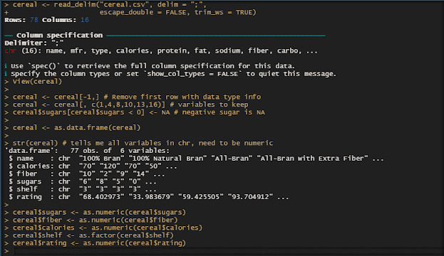
Hi everyone! Almost everyone starts their mornings with a nice bowl of cereal. In the grocery aisle, you choose a box of cheerios and chocolate puffs. However, your decision to buy that cereal may not have been completely your choice at all. You just picked from the options that were conveniently placed in front of you. My project will analyze the relationship between the shelves cereals are placed on to the sugar, fiber, and calories of that cereal. Do the ingredients of cereals, either healthy or sugary, play a role in what shelf cereals are placed on and their ratings? Two Part Analysis Do the ingredients s ugar, calories, and fiber content have a true mean difference with that cereal's placement on shelf 1,2, or 3 (counting from the ground)? I will use boxplots to understand each ingredients distribution in the shelves and perform ANOVA tests to determine if each ingredient is significant for the placement of the the cereal. ANOVA i...
Hi everyone! This week we dive into a more complex regression analysis than the linear regression we have done. Before we had one predictor variable and one outcome variable. In multivariate multiple regression, we have multiple predictor(or independent) variable but one outcome variables we are analyzing. The formula looks like y = b 1 x 1 + b 2 x 2 + … + b n x n + error. We will look into the relationships between the variables collectively using ANOVA analysis and individually through linear regression (lm) to understand which variables are contributing to the significance of the relationship. R sqaured will be an important factor to look into because it shows the amount of variation in dependent variable explained by the regression, thus a larger R squared indicates the predictor is more precisely able to predict outcome. 9.1. Conduct ANOVA (analysis of variance) and Regression coefficients to the data from cyst...


Comments
Post a Comment