Module 6: Normal life of Normal Distributions
Hi everyone!
A.
Consider a population consisting of the following values, which represents the number of ice cream purchases during the academic year for each of the five housemates.
8, 14, 16, 10, 11
a. Compute the mean of this population.

b. Select a random sample of size 2 out of the five members.
Sample is 16 and 8
c. Compute the mean and standard deviation of your sample.

d. Compare the Mean and Standard deviation of your sample to the entire population of this set (8,14, 16, 10, 11).

The mean of the population is 11.8, while the sample mean is 12. The standard deviation of the population is 2.856, while the sample standard deviation is 5.656. The spread is greater for the sample and the mean is relatively the same.
I created a function sd_pop() to find the standard deviation for the population because sd() uses n-1 which is for sample standard deviations.
B.
Suppose that the sample size n = 100 and the population proportion p = 0.95.
- Does the sample proportion p have approximately a normal distribution? Explain.
A. Population mean= (8+14+16+10+11)/ 5 = 11.8
B. Sample of size n= 5
C. Mean of sample distribution: 11.8
sample 1=
sample 2=
sample 3 and so on and so forth…
And Standard Error
(x-u)^2
Sum of last column = 40.8
Standard deviation of sample distribution = sqrt(40.8 / (5-1)) = 3.193
C.
From our textbook, Chapter 2 Probability Exercises # 2.4
Simulated coin tossing is probability better done using function called rbinom than using function called sample. Explain.
The function rbinom() requires a number of observations, number of trials, and the probability of success which in a coin toss matches the characteristics of a binomial distribution with only two mutually exclusive outcomes of heads or tails with identical trials. If we used the sample function there would be a needed vector x of values and the sample size. This function does not specify a need for probability of success and does not require mutually exclusive outcomes of pass or fail making it difficult to use with coin tossing.
-Ramya's POV


Comments
Post a Comment